Placer gold mining excavates and reworks riverbed sediments. At 10 m resolution it is visible to public optical satellites — Sentinel-2 in particular — but the resulting spectral disturbance must be separated from a large background of natural variation: seasonal phenology, snow cover, river migration, dust events, and inter-annual climate drift. Most remote-sensing pipelines for surface-mining detection fall into one of three families: (i) thresholded differencing of spectral indices between two dates or two seasonal composites; (ii) supervised classifiers trained on labelled imagery; and (iii) harmonic time-series decompositions (BFAST, CCDC, LandTrendr) that fit a periodic-plus-trend model to a per-pixel index series and flag deviations from it.
Two properties of Mongolian river basins constrain which of those families can be applied directly.
Irregular sampling. Sentinel-2 revisits the area on a fixed orbital cadence, but the usable record at each pixel is irregular. The Scene Classification Layer flags clouds, cloud shadows, cirrus, and snow; after masking, each pixel's time series has a multi-month gap every winter and shorter scattered gaps elsewhere. Algorithms that assume regular sampling — including the discrete Fourier transform — cannot be fit on this signal without first imputing values, and any imputation pre-determines what the model will later call an anomaly.
Large-amplitude seasonality. The steppe and its riparian corridors swing through a wide annual cycle: rapid green-up after snowmelt, summer drying, autumn bare-soil exposure, and a long snow-covered winter. The amplitude of these natural cycles is comparable in magnitude to the spectral change produced by mining. A single threshold applied to a date-pair difference therefore confuses seasonal swing for disturbance, and a model that adapts too quickly to recent observations will treat a freshly excavated cell as the "new normal" and stop flagging it.
Given those two constraints, three design choices structure the rest of the paper.
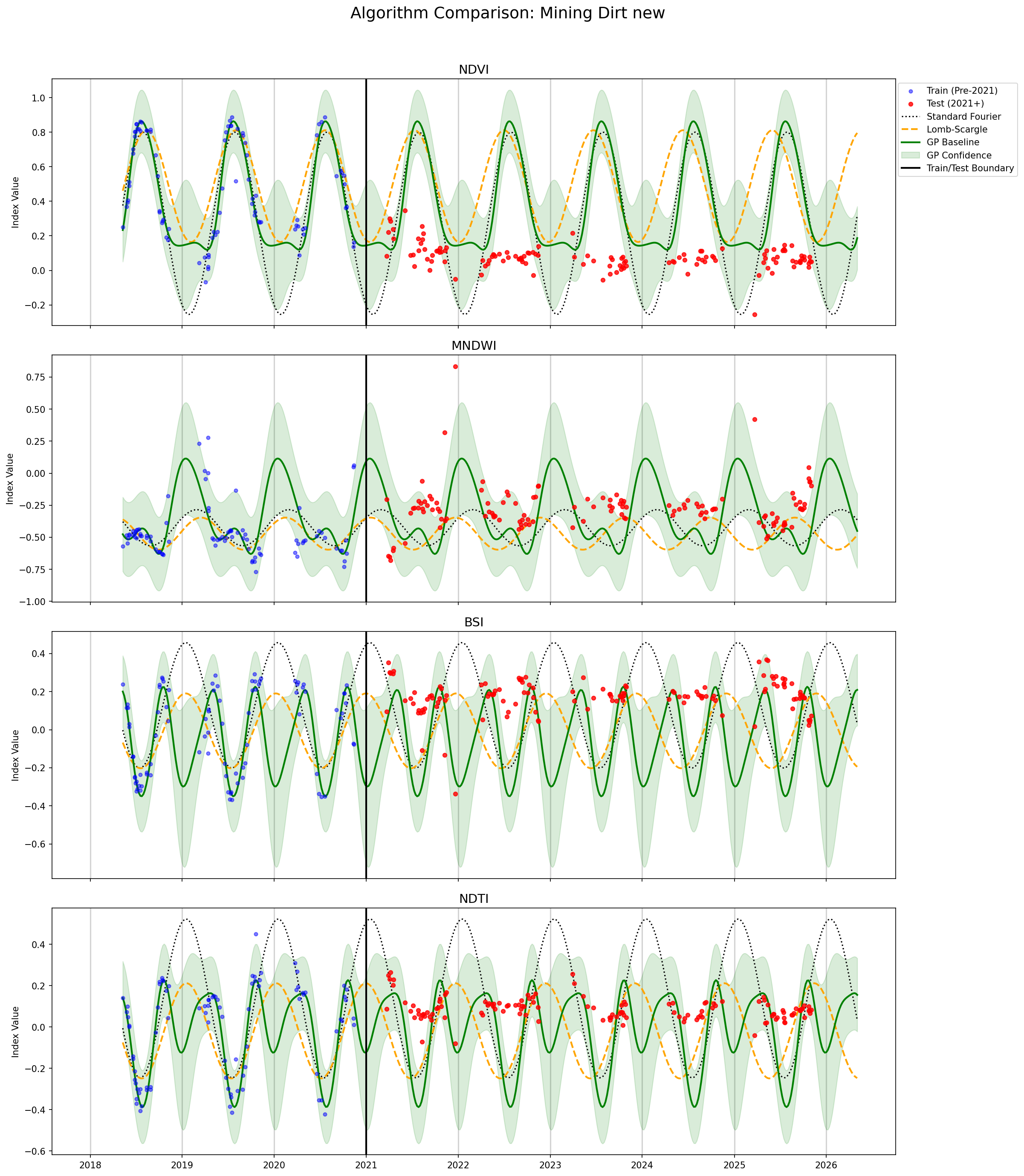
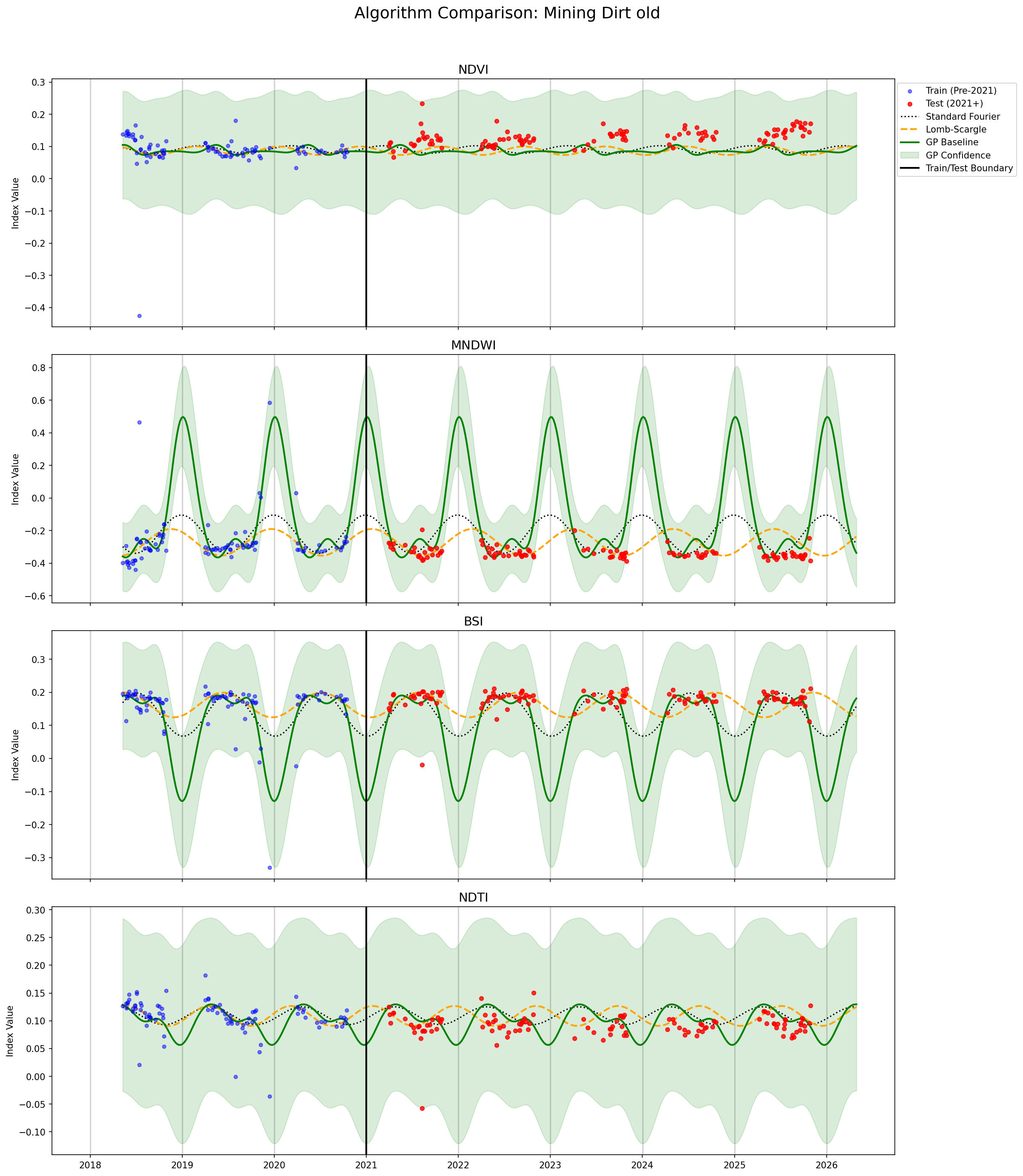
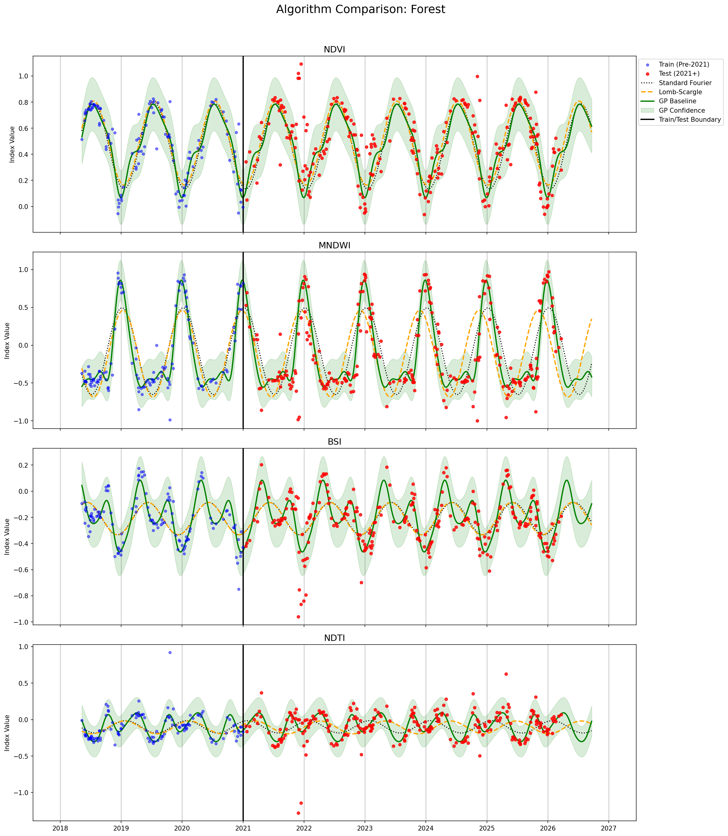
(a) Periodic harmonic filtering of the seasonal cycle. The seasonal component is the largest source of nuisance variance, and it is approximately one-period-per-year. The natural tool is harmonic regression — a sum of sines and cosines at the annual frequency. Because the raw record is irregularly sampled, ordinary least-squares Fourier fitting is not viable; the Lomb-Scargle periodogram and related variants handle uneven sampling but are not well suited to extracting a smooth baseline at arbitrary query dates. A Gaussian Process with a periodic covariance kernel provides the same harmonic decomposition in a form that natively tolerates gaps and returns a posterior mean at any timestamp.
(b) Constraints on the GP so that it does only what is asked. The GP is restricted to behave as a seasonal filter rather than a general curve-fitter: the periodic component's period is fixed at exactly one year, the trend component's lengthscale is fixed at five years (so the trend can absorb only slow climatic drift, not the step-like rupture caused by excavation), and the mean function is a learned constant rather than a flexible drift. The only quantities free to be learned per pixel are the two scale-kernel outputscales, the noise level, and the constant mean.
(c) Accumulated, multi-index evidence rather than per-date thresholds. Mining is persistent and shows up jointly across multiple physical indices. The pipeline therefore (i) computes standardised residuals for four indices (NDVI, BSI, MNDWI, NDTI), (ii) accumulates each into a leaky CUSUM whose decay rate corresponds to roughly one seasonal half-life, and (iii) fuses the four CUSUM cubes by elementwise minimum, so a pixel must be simultaneously anomalous on all four channels to enter the detection mask.
The input to the pipeline is a Sentinel-2 surface-reflectance cube over the area of interest, with one entry per acquisition date and six optical bands (blue, green, red, near-infrared, and two short-wave-infrared channels) plus the per-pixel Scene Classification Layer.
Each acquisition's classification layer is read in parallel with the optical bands. Pixels marked as no-data, saturated, cloud shadow, cloud (medium or high probability), cirrus, or snow are set to NaN in the optical bands. NaNs are propagated through the rest of the pipeline, not interpolated, so that gaps are visible to the model as missing observations rather than as smoothed-over guesses.
Four normalised difference indices are computed from the masked bands and carried through the rest of the pipeline:
They were chosen because mining produces a joint signature across the four (vegetation loss + bare soil + turbid ponds + sediment-laden runoff), whereas natural disturbances (floods, droughts, snow) excite the four in different combinations.
The seasonal baseline at each pixel is modelled as a Gaussian Process whose covariance is a sum of two scaled components:
with t measured in years from the start of the record. Three hyperparameters are fixed, not learned:
| Hyperparameter | Value | Role |
|---|---|---|
| Periodic period p | 1 year | Locks the periodic component to exactly one cycle per year. |
| Trend lengthscale ℓ | 5 years | Forces the trend component to vary only on multi-year scales. |
| Mean function | constant | A single learned constant per pixel — no flexible drift in the mean. |
The intent of these constraints, taken together, is that the GP can capture only two kinds of structure: an annual sinusoidal-like cycle and slow multi-year climatic drift. Anything else — including a step change caused by excavation — is forced into the residual, where it can be scored. If the trend lengthscale were small, or the mean function flexible, the GP would adapt to a freshly excavated pixel within a season or two and the disturbance would be absorbed into the baseline.
The only parameters free to be learned per pixel are the two outputscales (σ²per, σ²tr), the observation-noise variance, and the constant mean.
Exact Gaussian-Process inference is cubic in the number of training points, and the area of interest contains on the order of 310 000 pixels. The implementation exploits the fact that the number of valid (non-cloud, non-snow) observations differs across pixels but the linear-algebra structure is identical for any two pixels with the same valid count: pixels are grouped by their valid-observation count, each group is fitted in parallel on the GPU as a single batched problem of up to 2 048 pixels at a time, and posterior means and variances are evaluated in chunks of 50 dates. This bounds GPU memory to fit consumer-grade hardware and is purely a runtime optimisation — it does not change the mathematical model in §2.3.
The standardised anomaly score for each index, date, and pixel is
where:
direction = −1 is used for NDVI (since the diagnostic for vegetation loss is a negative residual) and +1 for the bare-soil, water, and turbidity indices.The effect of the empirical term is that each pixel is judged against its own historical envelope: a pixel whose pre-2021 residuals were noisy (an active river channel, for example) has a large σ²emp and produces small z-scores for the same physical change that would produce a large z-score on a previously stable pixel. The GP-variance term prevents the score from blowing up at dates where the GP itself is poorly constrained — for example, immediately after a long winter gap.
The per-date z-score is the evidence on a single observation. To convert it into evidence of persistent disturbance, a leaky cumulative sum (CUSUM) is applied independently to each index:
with a per-day decay of 0.99432, giving a half-life of ln 2 / ln(1/0.99432) ≈ 121 days — roughly one season. The accumulator is clamped at zero so that brief opposite-sign excursions do not produce negative debt that would mask a later real anomaly, and Δdi is the actual number of days between consecutive valid timestamps (so the boundary between training and inference windows is bridged with the true gap, not reset to zero). Cloud-masked timesteps contribute nothing to the sum, but the decay still applies, so an extended invalid stretch causes the accumulator to fade rather than freeze.
The four index-specific CUSUM cubes are then fused at each timestep by elementwise minimum:
and a pixel is reported as anomalous on date t if and only if Cfused > 6. Because the minimum is taken pointwise across indices, no single channel can carry the score above threshold on its own; agreement across all four physical indices is required.
At each timestamp in the record, the binary mask of pixels with fused score above the threshold is vectorised into polygons and reprojected to geographic coordinates, producing one set of detection polygons per acquisition date. The full series of per-date polygons is what the demo front-end renders on the map.
Quantitative numbers (counts of detection dates, total flagged area, and timing of disturbance onsets) are to be filled in once the validation pass against the digitised reference is complete.
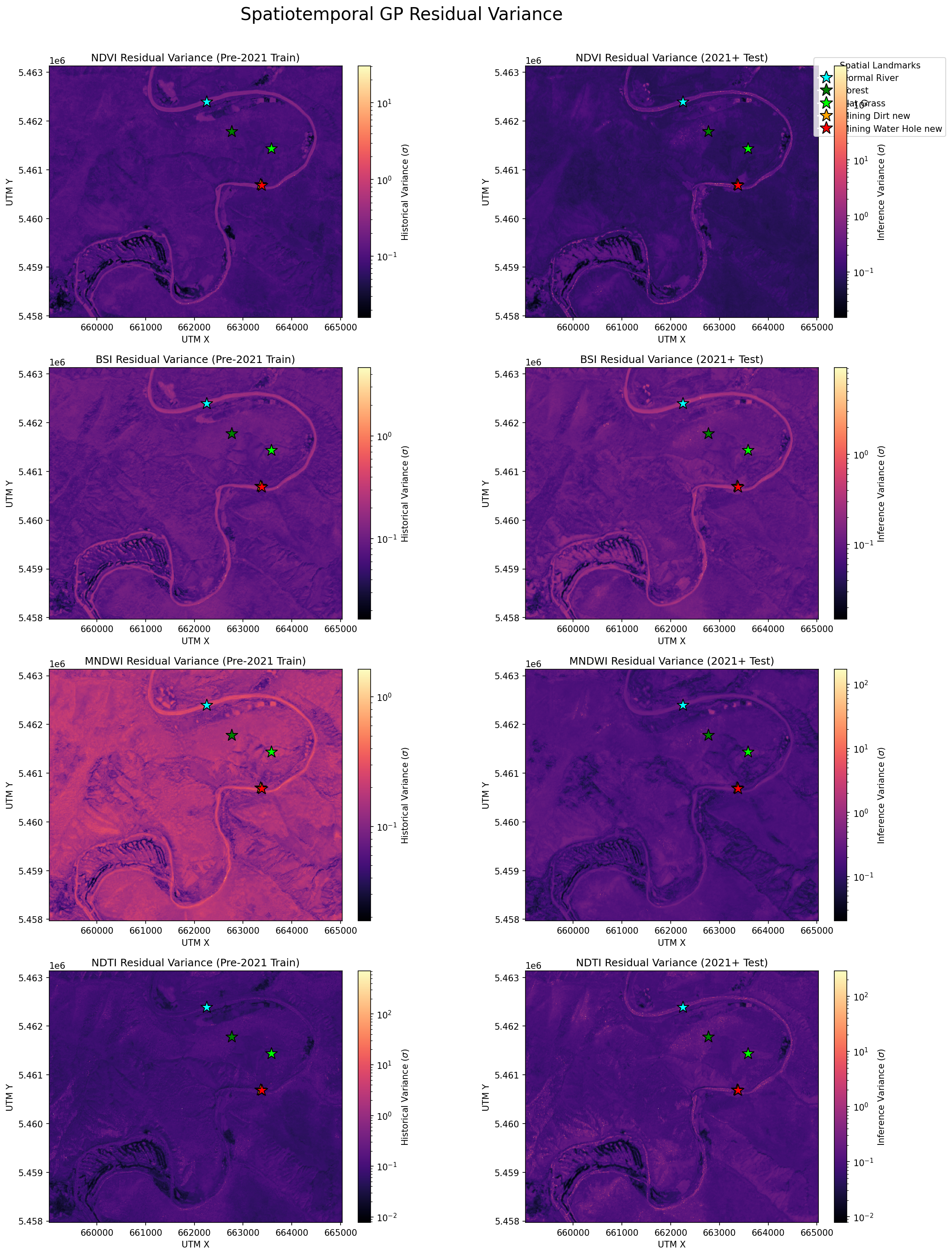
The fitted baseline was inspected at seven hand-chosen reference points covering the main land-cover and disturbance classes in the area: a stretch of natural river, a forested patch, an undisturbed flat-grass patch, two recent mining sites (dry pit and water-filled pit), and two older mining sites that were already disturbed before the training cut-off. Three distinct patterns are observed across these classes:
The two-dimensional map of σ̂emp over the area of interest is brightest along the active river channel and its floodplain and dim over the surrounding steppe — the geometry expected from §2.5. The interesting consequence is in the final detection layer rather than in the variance map itself. Along the river shore, the per-date z-score does occasionally rise, because river meanders shift and vehicle tracks appear along access roads. But at the 10 m pixel scale, the natural curling of the channel is a small geometric change relative to σ̂emp, and the river-shore z-scores rarely accumulate to the fused threshold. Detections that do appear in the riparian band are concentrated at points consistent with ground disturbance — excavation pits and access tracks — rather than tracking the river edge itself.
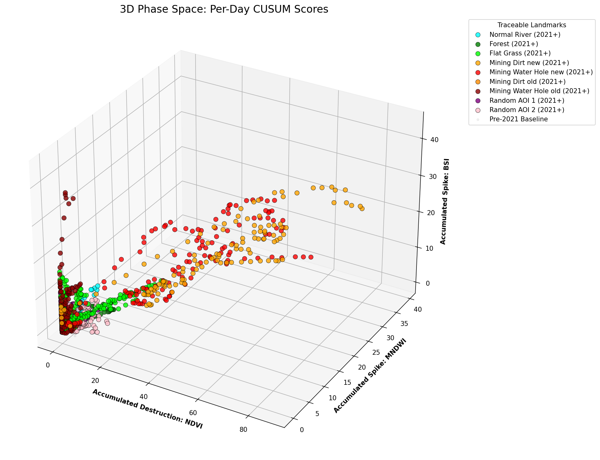
The 3D scatter of (CNDVI, CMNDWI, CBSI) — the per-index leaky CUSUM trajectories defined in §2.6 — coloured by the reference-point classes shows that mining pixels occupy a region of phase space distinct from natural river and forest pixels: large CNDVI co-occurring with large CBSI and elevated CMNDWI. Natural river pixels lie along a different axis (elevated CMNDWI without the BSI signature). This separation is the empirical justification for the strict-AND fusion in §2.6.
The pipeline produces one set of detection polygons per acquisition date across the full inference window. Reported per year: the number of dates carrying at least one detection polygon, the total area flagged, and the spatial concentration of detections along the active corridor (Table 1, to be inserted).
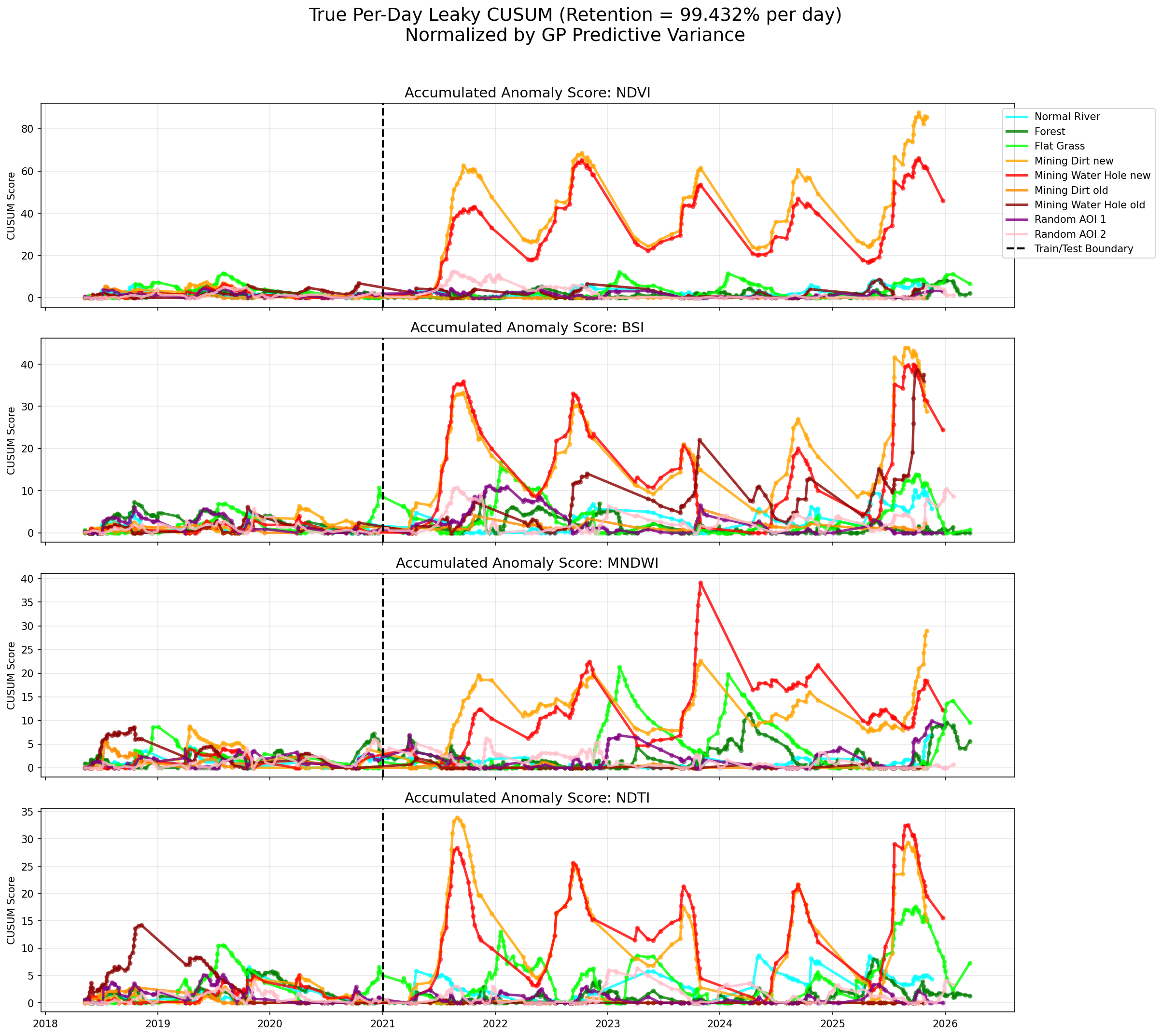
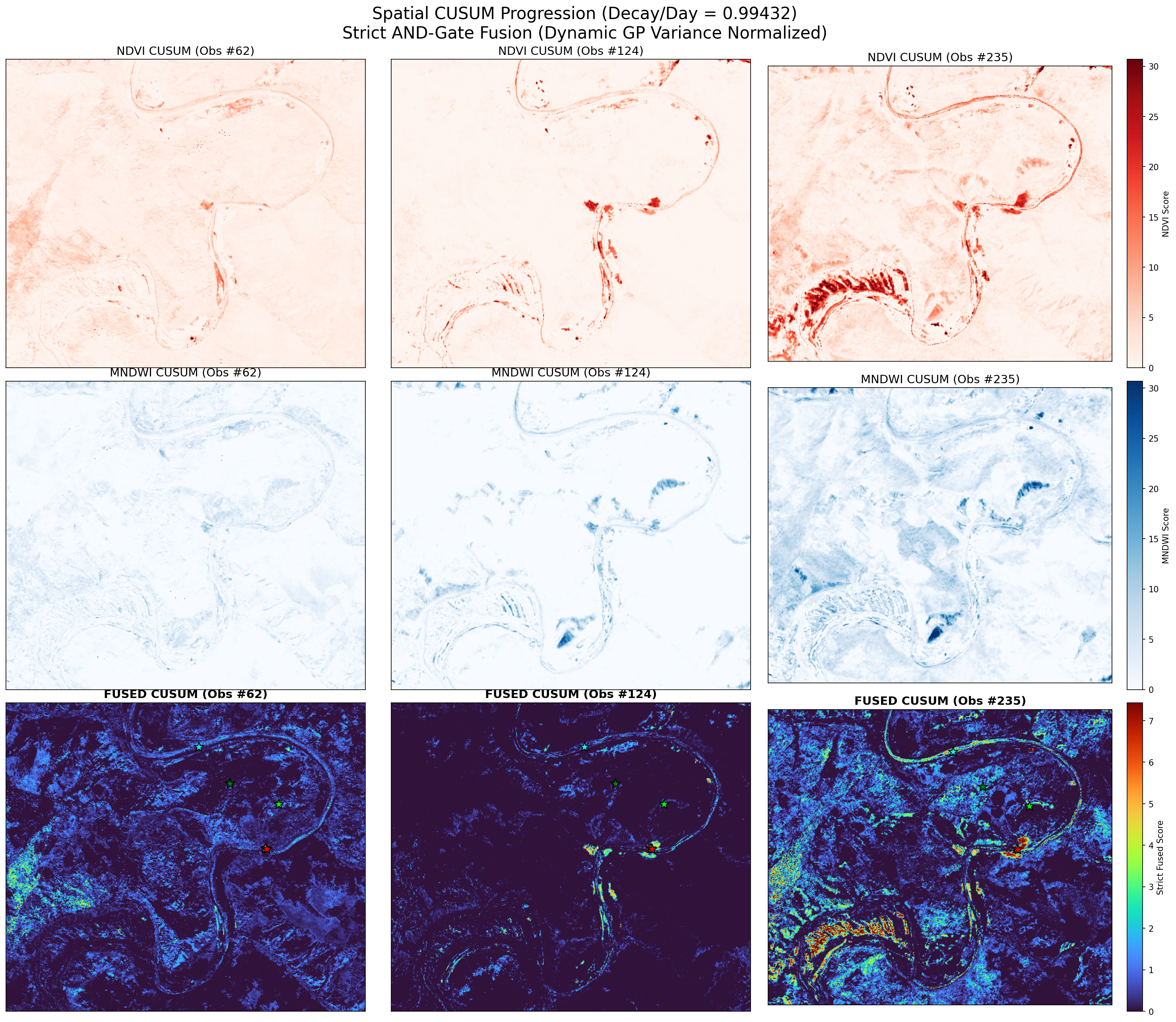
The full-AOI output of the pipeline is illustrated at three representative dates spanning the train/test boundary. The fused score shown is the strict elementwise minimum across the four index-specific CUSUM cubes (§2.6), normalised by the dynamic GP predictive variance (§2.5). Pre-2021 slices stay near zero almost everywhere; post-2021 slices concentrate elevated fused scores along the active mining corridor. Reading the colour scale across the three panels, fused values above ≈5–6 reliably correspond to spatially coherent disturbance, while smaller values mostly populate noisy riparian pixels that fail to accumulate. This empirical separation is what fixes the §2.6 detection threshold of 6 on the fused score.